平滑曲線
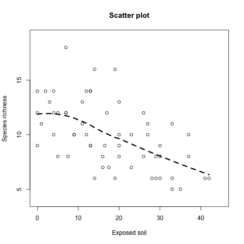
在上面的圖形中,由於整個資料沒有很明顯的趨勢,這時候可以利用 loess 配適一條平滑曲線,幫助我們更容易抓出整個資料大概的走勢:
plot(x = Veg$BARESOIL, y = Veg$R,
  xlab = "Exposed soil",
  ylab = "Species richness", main = "Scatter plot",
  xlim = c(0, 45), ylim = c(4, 19))
M.Loess <- loess(R ~ BARESOIL, data = Veg)
Fit <- fitted(M.Loess)
Ord1 <- order(Veg$BARESOIL)
lines(Veg$BARESOIL[Ord1], Fit[Ord1],
  lwd = 3, lty = 2)
Exercise 1
Amphibian_road_Kills.xls 是兩棲動物在葡萄牙馬路上的死亡資料,TOT.N 是該觀測點動物的死亡數,而 OLIVE 是橄欖樹的數量,D.PARK 則是觀測點到最近的自然公園之間的距離。
請將 Amphibian_road_Kills.xls 的資料讀入 R,並且依序進行下列動作:
- 畫出
TOT.N與D.PARK的關係圖,並加入適當的文字標示。 - 使用資料點的大小來表示
OLIVE的數量。 - 加入平滑曲線。
總覽
下面這張表是本篇所介紹過的 R 函數總覽。
| 函數 | 說明 | 範例 |
|---|---|---|
plot |
畫出 x 與 y 的分佈圖(scatter plot)。 |
plot (x, y) |
lines |
在圖形中加入線條。 | lines (x, y) |
order |
計算資料的排序向量。 | order(x) |
loess |
LOESS 平滑曲線。 | M <- loess (y ~ x) |
fitted |
計算配適值。 | fitted (M) |