資料點顏色
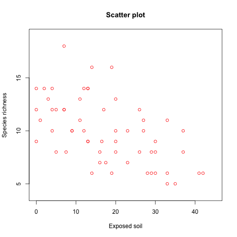
使用不同的顏色來表示不同的資料也是常見的繪圖方式,資料點的顏色是用 col 參數來指定的:
plot(x = Veg$BARESOIL, y = Veg$R,
  xlab = "Exposed soil",
  ylab = "Species richness", main = "Scatter plot",
  xlim = c(0, 45), ylim = c(4, 19),
  col = 2)
畫出來的圖形為
col 指定的整數會透過 palette 對應到實際使用的顏色,我們可以執行 palette 查看目前的顏色對應:
palette()
預設的輸出為
[1] "black"   "red"     "green3"  "blue"
[5] "cyan"    "magenta" "yellow"  "gray"
編號 1 對應到的顏色是黑色,編號 2 則是紅色,以此類推。另外 col 還可以使用很多種方式指定顏色,詳細說明請參考 par 的線上手冊。
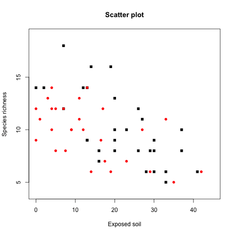
col 跟 pch 的使用方式類似,也都可以靠著向量的方式指定個別資料點的顏色,假設我們要將 1974 年以前的資料用黑色實心的方塊表示,而其餘的資料則用紅色實心的圓圈表示,可以這樣做:
Veg$Time2 <- Veg$Time
Veg$Time2 [Veg$Time <= 1974] <- 15
Veg$Time2 [Veg$Time > 1974] <- 16
Veg$Col2 <- Veg$Time
Veg$Col2 [Veg$Time <= 1974] <- 1
Veg$Col2 [Veg$Time > 1974] <- 2
plot(x = Veg$BARESOIL, y = Veg$R,
  xlab = "Exposed soil",
  ylab = "Species richness", main = "Scatter plot",
  xlim = c(0, 45), ylim = c(4, 19),
  pch = Veg$Time2, col = Veg$Col2)
畫出來的圖形為
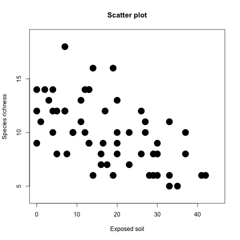
資料點大小
圖形中資料點的大小可以使用 cex 參數來指定,其預設值是 1,若指定為 2.5 的話,所有的資料點就會變成原來的 2.5 倍大:
plot(x = Veg$BARESOIL, y = Veg$R,
  xlab = "Exposed soil", ylab = "Species richness",
  main = "Scatter plot",
  xlim = c(0, 45), ylim = c(4, 19),
  pch = 16, cex = 2.5)
畫出來的圖形為
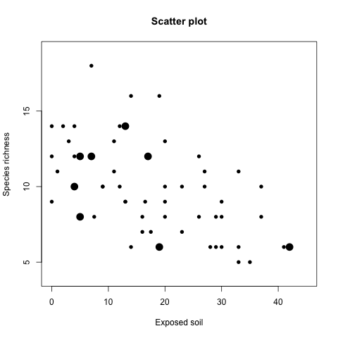
cex 同樣也可以使用向量的方式指定個別的資料點:
Veg$Cex2 <- Veg$Time
Veg$Cex2[Veg$Time == 2002] <- 2
Veg$Cex2[Veg$Time != 2002] <- 1
plot(x = Veg$BARESOIL, y = Veg$R,
  xlab = "Exposed soil", ylab = "Species richness",
  main = "Scatter plot",
  xlim = c(0, 45), ylim = c(4, 19),
  pch = 16, cex = Veg$Cex2)
畫出來的圖形為