這裡介紹如何在 R 中的使用各種機率分佈以及基本模型配適方法。
資料的基本統計量以及各種圖形對於資料的了解有很大的幫助,但這兩種方式在資料比較複雜的狀況下會有些問題,例如當變數的數量很多時,基本的統計量無法呈現資料的詳細分布狀況,而太多的圖形則會使人難以理解,另外也無法對於未來的資料做預測。
如果我們對於資料的結構與特性有足夠的了解,就可以使用適當的統計模型來配適資料,並且使用配適出來的模型進行資料的預測,而在進行模型配適之前,我們必須先對基本的隨機變數與機率分佈有所認識。
隨機變數
隨機變數對於許多的應用來說都是很重要的,R 中也內建非常多的隨機變數產生函數,可以生成各種分佈的隨機變數。
sample 函數
sample 是一個用來產生隨機變數的函數,但是它的使用方式比較特殊。如果只指定單一個整數的參數 n,它會傳回從 1 到 n 的隨機排列組合:
sample(6)
[1] 3 4 2 5 1 6
如果指定兩個整數參數 n 與 m,則會產生 m 個介於 1 到 n 的隨機整數:
sample(6, 3)
[1] 3 4 2
在預設的狀況下,sample 會以取後不放回的方式產生隨機變數,所以每一個產生的數字都會不同,若要以後放回的方式產生隨機變數,可以加上 replace = TRUE 參數:
sample(6, 8, replace = TRUE)
[1] 2 6 1 2 2 5 2 1
sample 最常被使用的功能就是隨機抽樣,它可以從既有的向量中隨機取出樣本:
x <- c(1.2, 4.5, 6.3, 9.1, 4.6, 8.4, 5.9, 1.8)
sample(x, 5)
[1] 4.6 4.5 1.8 6.3 5.9
除了數值資料外,其他各種的向量也都可以使用 sample 來做隨機抽樣。我們以內建的 letters 做示範,這個內建的向量中包含 26 個英文字母,若要從中隨機取出 5 個英文字母,可以使用 sample 函數來處理:
sample(letters, 5)
[1] "r" "i" "x" "o" "p"
sample 在隨機取樣時,也可以使用 prob 參數指定每個元素的權重:
weights <- c(1, 1, 2, 3, 5, 8, 13, 21, 8, 3, 1, 1)
sample(month.abb, 3, prob = weights)
[1] "Aug" "May" "Jul"
機率分佈
R 可以產生數十種分佈的隨機變數,一般常見的隨機分佈 R 都有支援,我們可以查詢 distribution 的線上說明文件:
?distribution
另外在 R 的官方網站上也有很詳盡的說明。
大部分 R 的隨機變數產生函數都會以 r 字母開頭(r 代表隨機變數產生器 ,random number generator),然後加上分佈的名稱來作為函數的名稱,例如 runif 就是產生均勻分佈(uniform distribution)隨機變數的函數,而 rnorm 函數則會產生常態分佈(normal distribution)的隨機變數。通常這類產生隨機變數的函數,其第一個參數是指定要產生的隨機變數數量,而後續的參數則是各分佈的參數,例如產生五個介於 0 與 1 的均勻分佈隨機變數:
runif(5)
[1] 0.9228195 0.8629326 0.2507834 0.7132745 0.7286481
產生五個介於 2 與 10 的均勻分佈隨機變數:
runif(5, 2, 10)
[1] 4.601491 8.254266 8.853793 3.272245 5.628698
產生五個標準常態分佈的隨機變數:
rnorm(5)
[1] 0.9256513 -1.7038184 1.1460961 -1.2906661 -0.1514443
產生五個平均值為 3,標準差為 8 的常態分佈隨機變數:
rnorm(5, 3, 8)
[1] -2.459081 -5.538817 -6.284891 4.256028 6.398596
偽隨機變數產生器
R 的隨機變數生成跟一般的軟體一樣都是使用偽隨機(pseudorandom)的方式,R 支援好幾種隨機變數產生方法(包含平行化的隨機變數產生),詳細說明可以參考 RNG的線上說明:
?RNG
若需要其他不同的隨機變數產生演算法,可以參考 R 的官方網站。
若要查詢目前所使用的隨機變數產生方法,可以使用 RNGkind 函數查詢:
RNGkind()
[1] "Mersenne-Twister" "Inversion"
隨機變數產生器在產生隨機變數時,都會需要指定一個亂數種子(random seed),使用同樣的亂數種子就可以產生一樣的隨機亂數,在 R 中我們可以使用 set.seed 函數來指定亂數種子:
set.seed(1)
runif(5)
[1] 0.2655087 0.3721239 0.5728534 0.9082078 0.2016819
set.seed(1)
runif(5)
[1] 0.2655087 0.3721239 0.5728534 0.9082078 0.2016819
set.seed 所接受的參數是一個正整數,至於該正整數的數值是多少並不重要,重點只在於使用同樣的亂數種子就可以產生相同的亂數,確保程式每次執行的結果都會相同,這個技巧在程式的開發與驗證上相當重要。
機率分佈
除了隨機變數的生成之外,對於大部分的機率分佈 R 同時也提供一系列的機率相關函數,例如機率密度函數(probability density function,簡稱 PDF)、累積密度函數(cumulative density function,簡稱 CDF)以及 CDF 的反函數,這些函數的命名規則跟產生隨機變數的函數類似:
r開頭:產生隨機變數,例如rnorm。d開頭:機率密度函數,例如dnorm。p開頭:累積密度函數,例如pnorm。q開頭:CDF 的反函數,例如qnorm。
公式
R 的公式(formula)是一種特殊的語法,用來表示由變數所構成的模型,至於實際上所代表的意義則會跟使用模型的函數有關。
我們以 iris 這個 R 內建的資料集做示範,假設我們有一個迴歸模型如下:
若使用 R 的公式表示則為:
Sepal.Length ~ Sepal.Width + Petal.Width + Petal.Length
公式的左側是擺放反應變數(response variable)而右側則是放解釋變數(explanatory variables),中間以一個 ~ 符號區隔,而右側若有多個解釋變數,則使用加號 + 分隔,這樣就是一個最簡單的線性模型。
若要指定沒有截距項的模型:
\[ \begin{aligned} \mbox{Sepal.Length} = & \beta_1 \mbox{Sepal.Width} + \\ & \beta_2 \mbox{Petal.Width} + \beta_3 \mbox{Petal.Length} + \epsilon \end{aligned} \]則可以在右側加上一個 0,這樣就代表不包含截距項的模型:
Sepal.Length ~ 0 + Sepal.Width + Petal.Width + Petal.Length
下表是常用於 R 公式中的各種符號與意義。
| 符號 | 意義 |
|---|---|
~ | 分隔反應變數(左側)與解釋變數(右側)。 |
+ | 分隔多個解釋變數。 |
: | 代表解釋變數之間的交互作用,例如 y ~ x + z + x:z 就代表除了以 x 與 z 解釋 y 之外,還加入了 x 與 z 兩個變量的交互作用。 |
* | 代表所有可能的交互作用,例如 y ~ x * z * w 就等同於 y ~ x + z + w + x:z + x:w + z:w + x:z:w。 |
^ | 以次方表示變數之間的交互作用,例如 y ~ (x + z + w)^2 就等同於 y ~ x + z + w + x:z + x:w + z:w。 |
. | 代表除了反應變數之外,data frame 中所有的變數,假設整個 data frame 中包含 x、y、z 與 w ,則 y ~ . 就代表 y ~ x + z + w。 |
- | 減號代表從現有的模型中移除指定的解釋變數,例如 y ~ (x + z + w)^2 – x:w 就代表 y ~ x + z + w + x:z + z:w。 |
-1 | 移除截距項,例如 y ~ x - 1。 |
+0 | 移除截距項,與 -1 相同,例如 y ~ x + 0 或 y ~ 0 + x。 |
I() | 以數學意義解釋,例如一般的 y ~ x + (z + w)^2 會等同於 y ~ x + z + w + z:w,而 y ~ x + I((z + w)^2) 則會等同於 y ~ x + h,其中這個 h 是一個新建立的變數,其值為 z 與 w 總和的平方,亦即 (h = (z + w)^2)。 |
| 一般函數 | 一般的數學函數都可以直接用在公式中,例如 log(y) ~ x + z + w。 |
線性迴歸模型
線性迴歸模型是最簡單的迴歸模型,它可以使用公式指定迴歸模型,並指定資料來源的 data frame,例如:
iris.lm <- lm(Petal.Width ~ Petal.Length, data = iris)
iris.lm
Call:
lm(formula = Petal.Width ~ Petal.Length, data = iris)

Coefficients:
 (Intercept)  Petal.Length
     -0.3631        0.4158
這樣就完成最簡單的線性迴歸模型配適。
以 lm 配適所得到的結果,可以使用以下這些函數來顯示更詳細的資訊,或做進一步的分析:
| 函數 | 功能 |
|---|---|
summary() | 顯示詳細的模型配適結果。 |
coefficients() | 顯示模型的迴歸係數,包含截距項與各解釋變數的係數。 |
confint() | 計算迴歸係數的區間估計值,預設會計算 95% 的信賴區間。 |
fitted() | 根據模型計算配適值。 |
residuals() | 根據模型計算殘差值。 |
anova() | 計算變異數分析(ANOVA)表格。 |
vcov() | 計算模型參數的變異數矩陣(covariance matrix)。 |
AIC() | 計算模型的 AIC(Akaike’s Information Criterion)值。 |
plot() | 畫出模型診斷用的各種圖形。 |
predict() | 以配適出來的模型,對新的資料進行預測。 |
coefficients 可顯示配適出來的迴歸係數:
coefficients(iris.lm)
(Intercept) Petal.Length
  -0.3630755    0.4157554
使用 summary 可以顯示更詳細一點的資訊:
summary(iris.lm)
Call:
lm(formula = Petal.Width ~ Petal.Length, data = iris)

Residuals:
     Min       1Q   Median       3Q      Max
-0.56515 -0.12358 -0.01898  0.13288  0.64272

Coefficients:
              Estimate Std. Error t value Pr(>|t|)
(Intercept)  -0.363076   0.039762  -9.131  4.7e-16 ***
Petal.Length  0.415755   0.009582  43.387  < 2e-16 ***
---
Signif. codes:  0 ‘***’ 0.001 ‘**’ 0.01 ‘*’ 0.05 ‘.’ 0.1 ‘ ’ 1

Residual standard error: 0.2065 on 148 degrees of freedom
Multiple R-squared:  0.9271,	Adjusted R-squared:  0.9266
F-statistic:  1882 on 1 and 148 DF,  p-value: < 2.2e-16
列出模型的配適值:
head(iris$Petal.Width)
1         2         3         4         5         6
0.2189821 0.2189821 0.1774065 0.2605576 0.2189821 0.3437087
與實際值做比較:
head(fitted(iris.lm))
[1] 0.2 0.2 0.2 0.2 0.2 0.4
列出殘差值:
head(residuals(iris.lm))
1           2           3           4           5           6
-0.01898206 -0.01898206  0.02259348 -0.06055760 -0.01898206  0.05629131
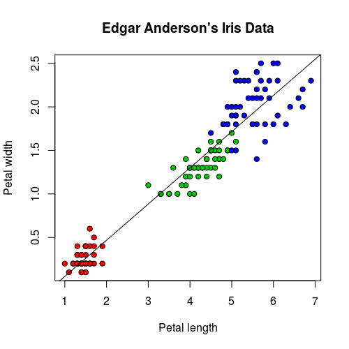
對於變數不多的模型,我們可以畫出其迴歸線與資料的圖形:
plot(iris$Petal.Length, iris$Petal.Width, pch=21,
  bg = c("red", "green3", "blue")[unclass(iris$Species)],
  main = "Edgar Anderson's Iris Data",
  xlab = "Petal length", ylab="Petal width")
abline(iris.lm$coefficients, col = "black")
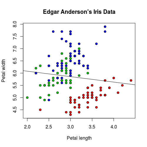
有時候基本的線性模型可能會無法準確地解釋資料,我們來看 Sepal.Length 與 Sepal.Width 之間的關係:
iris.lm2 <- lm(Sepal.Length ~ Sepal.Width, data = iris)
plot(iris$Sepal.Width, iris$Sepal.Length, pch=21,
  bg = c("red", "green3", "blue")[unclass(iris$Species)],
  main = "Edgar Anderson's Iris Data",
  xlab = "Petal length", ylab="Petal width")
abline(iris.lm2$coefficients, col = "black")
這是 Sepal.Length 與 Sepal.Width 的迴歸線,直接從圖形上看起來就可以發現這個模型配適的不太好。
若從 p-value 來看,結果也是一樣不好:
summary(iris.lm2)
Call:
lm(formula = Sepal.Length ~ Sepal.Width, data = iris)

Residuals:
    Min      1Q  Median      3Q     Max
-1.5561 -0.6333 -0.1120  0.5579  2.2226

Coefficients:
            Estimate Std. Error t value Pr(>|t|)
(Intercept)   6.5262     0.4789   13.63
這種狀況若將資料依據 Species 分組,再使用迴歸線配適,結果就會比較好:
iris.lm2 <- lm(Sepal.Length ~ Sepal.Width, data = iris)
iris.setosa.lm2 <- lm(Sepal.Length ~ Sepal.Width, data = iris[which(iris$Species=="setosa"),])
iris.versicolor.lm2 <- lm(Sepal.Length ~ Sepal.Width, data = iris[which(iris$Species=="versicolor"),])
iris.virginica.lm2 <- lm(Sepal.Length ~ Sepal.Width, data = iris[which(iris$Species=="virginica"),])
plot(iris$Sepal.Width, iris$Sepal.Length, pch=21,
  bg = c("red", "green3", "blue")[unclass(iris$Species)],
  main = "Edgar Anderson's Iris Data",
  xlab = "Petal length", ylab="Petal width")
abline(iris.lm2$coefficients, col = "black")
abline(iris.setosa.lm2$coefficients, col = "red")
abline(iris.versicolor.lm2$coefficients, col = "green3")
abline(iris.virginica.lm2$coefficients, col = "blue")
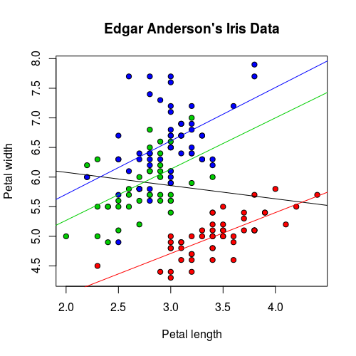
這樣三組資料所配適的模型都相當顯著。
summary(iris.setosa.lm2)
Call:
lm(formula = Sepal.Length ~ Sepal.Width, data = iris[which(iris$Species ==
    "setosa"), ])

Residuals:
     Min       1Q   Median       3Q      Max
-0.52476 -0.16286  0.02166  0.13833  0.44428

Coefficients:
            Estimate Std. Error t value Pr(>|t|)
(Intercept)   2.6390     0.3100   8.513 3.74e-11 ***
Sepal.Width   0.6905     0.0899   7.681 6.71e-10 ***
---
Signif. codes:  0 ‘***’ 0.001 ‘**’ 0.01 ‘*’ 0.05 ‘.’ 0.1 ‘ ’ 1

Residual standard error: 0.2385 on 48 degrees of freedom
Multiple R-squared:  0.5514,	Adjusted R-squared:  0.542
F-statistic: 58.99 on 1 and 48 DF, p-value: 6.71e-10summary(iris.versicolor.lm2)
Call:
lm(formula = Sepal.Length ~ Sepal.Width, data = iris[which(iris$Species ==
    "versicolor"), ])

Residuals:
     Min       1Q   Median       3Q      Max
-0.73497 -0.28556 -0.07544  0.43666  0.83805

Coefficients:
            Estimate Std. Error t value Pr(>|t|)
(Intercept)   3.5397     0.5629   6.289 9.07e-08 ***
Sepal.Width   0.8651     0.2019   4.284 8.77e-05 ***
---
Signif. codes:  0 ‘***’ 0.001 ‘**’ 0.01 ‘*’ 0.05 ‘.’ 0.1 ‘ ’ 1

Residual standard error: 0.4436 on 48 degrees of freedom
Multiple R-squared:  0.2766,	Adjusted R-squared:  0.2615
F-statistic: 18.35 on 1 and 48 DF, p-value: 8.772e-05summary(iris.virginica.lm2)
Call:
lm(formula = Sepal.Length ~ Sepal.Width, data = iris[which(iris$Species ==
    "virginica"), ])

Residuals:
     Min       1Q   Median       3Q      Max
-1.26067 -0.36921 -0.03606  0.19841  1.44917

Coefficients:
            Estimate Std. Error t value Pr(>|t|)
(Intercept)   3.9068     0.7571   5.161 4.66e-06 ***
Sepal.Width   0.9015     0.2531   3.562 0.000843 ***
---
Signif. codes:  0 ‘***’ 0.001 ‘**’ 0.01 ‘*’ 0.05 ‘.’ 0.1 ‘ ’ 1

Residual standard error: 0.5714 on 48 degrees of freedom
Multiple R-squared:  0.2091,	Adjusted R-squared:  0.1926
F-statistic: 12.69 on 1 and 48 DF,  p-value: 0.0008435
像上面這樣將資料分組之後,再進行配適的模型,可以使用這樣的公式表示:
Sepal.Length ~ Sepal.Width:Species + Species - 1
使用 lm 配適的結果完全相同:
iris.lm3 <- lm(Sepal.Length ~ Sepal.Width:Species + Species - 1, data = iris)
iris.lm3
Call:
lm(formula = Sepal.Length ~ Sepal.Width:Species + Species - 1,
    data = iris)

Coefficients:
                Speciessetosa              Speciesversicolor               Speciesvirginica
                       2.6390                         3.5397                         3.9068
    Sepal.Width:Speciessetosa  Sepal.Width:Speciesversicolor   Sepal.Width:Speciesvirginica
                       0.6905                         0.8651                         0.9015
由於 Species 是類別型的資料(R 的因子變數),無法直接用於迴歸模型的中,所以 R 會自動依據 Species 建立一些虛擬變數(dummy variables),讓它可以被用於迴歸模型中:
Speciessetosa:若Species為setosa則其值為1,否則為0。Speciesversicolor:若Species為versicolor則其值為1,否則為0。Speciesvirginica:若Species為virginica則其值為1,否則為0。Sepal.Width:Speciessetosa:若Species為setosa則其值為Sepal.Width,否則為0。Sepal.Width:Speciesversicolor:若Species為versicolor則其值為Sepal.Width,否則為0。Sepal.Width:Speciesvirginica:若Species為virginica則其值為Sepal.Width,否則為0。
使用 summary 顯示詳細的結果:
summary(iris.lm3)
Call:
lm(formula = Sepal.Length ~ Sepal.Width:Species + Species - 1,
    data = iris)

Residuals:
     Min       1Q   Median       3Q      Max
-1.26067 -0.25861 -0.03305  0.18929  1.44917

Coefficients:
                              Estimate Std. Error t value Pr(>|t|)
Speciessetosa                   2.6390     0.5715   4.618 8.53e-06 ***
Speciesversicolor               3.5397     0.5580   6.343 2.74e-09 ***
Speciesvirginica                3.9068     0.5827   6.705 4.25e-10 ***
Sepal.Width:Speciessetosa       0.6905     0.1657   4.166 5.31e-05 ***
Sepal.Width:Speciesversicolor   0.8651     0.2002   4.321 2.88e-05 ***
Sepal.Width:Speciesvirginica    0.9015     0.1948   4.628 8.16e-06 ***
---
Signif. codes:  0 ‘***’ 0.001 ‘**’ 0.01 ‘*’ 0.05 ‘.’ 0.1 ‘ ’ 1

Residual standard error: 0.4397 on 144 degrees of freedom
Multiple R-squared:  0.9947,	Adjusted R-squared:  0.9944
F-statistic:  4478 on 6 and 144 DF,  p-value: < 2.2e-16