Wikipedia 是一個全世界人都在使用的百科全書,我們可以從 Wikipedia 上面各個主題的使用狀況來分析出一些有趣的結果,例如軟體的普及程度等,另外也可以用來作為判斷軟體是否具有發展性的一個參考。
這裡我們針對矩陣計算軟體、作業系統等議題,分別使用 R 來抓取 Wikipedia 上面的使用資訊,並畫出圖表來分析,看看這些領域目前的情況。
矩陣計算軟體
首先來看 R 軟體本身的情況,下面這張是 R 語言近幾年在 Wikipedia 上面被查詢的狀況:
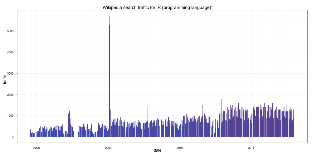
由這張圖可以看出來在這幾年中對 R 語言有興趣的人有成長的趨勢,而在 2009 年一月份因為紐約時報登了一篇關於 R 的文章,所以當月的瀏覽量突然暴增,由於增加的量相當驚人,原作者還一度以為是 bug。
接下來我們再來看看 Octave 與 Scilab 兩個軟體的情況,這兩個軟體也是跟 R 很類似的軟體,首先是 Octave:
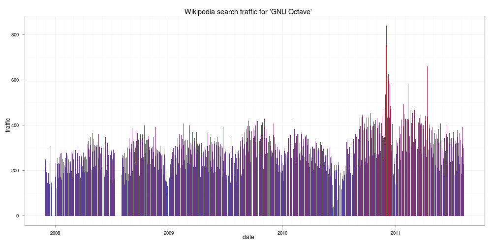
由圖中情況看起來,似乎對 Octave 有興趣的人沒有 R 來的多,再來看看 Scilab:
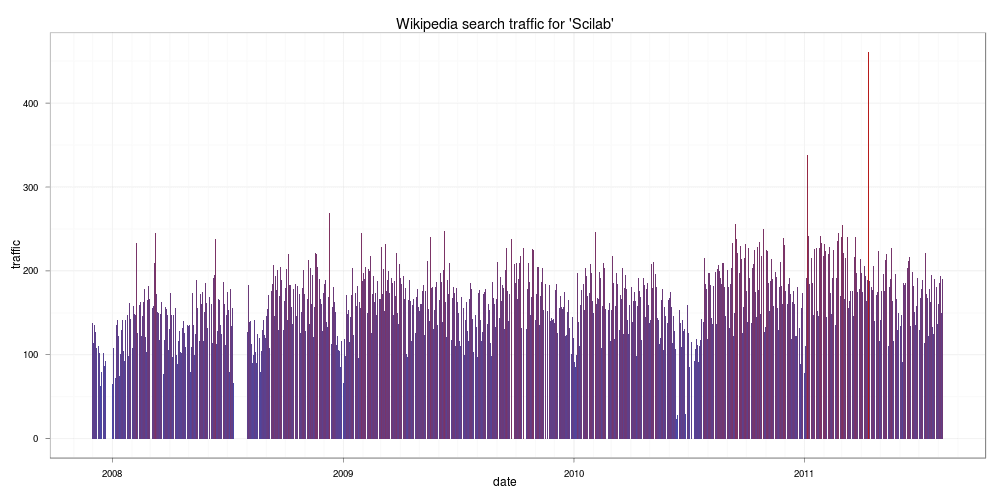
看起來比 Octave 更慘,如果您正在考慮學習哪一種矩陣計算工具,這個結果值得參考一下,畢竟使用者的多寡對於軟體的發展有一定的影響力,使用者太少的軟體,其發展與除錯的速度相對的會比較遲緩。
作業系統
首先來看最近很熱門的 Android:
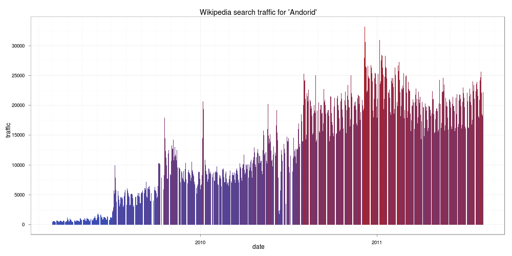
看來從 Google 一推出後,對於 Android 有興趣的人不斷上升,到了 2011 之後,似乎增加的速減緩了。接著來看 Linux:
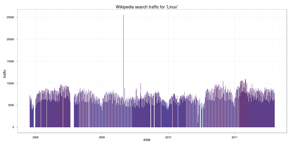
看起來都是很穩定的樣子。跟 Linux 很像的 FreeBSD:
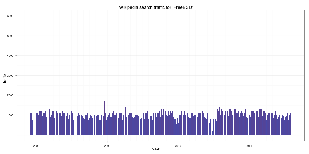
也是很穩定沒什麼變化,但是跟 Linux 比起來就差一大截。接著看一下微軟的 Windows:
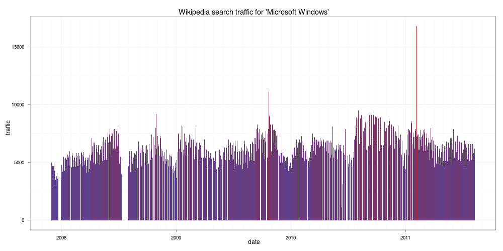
可能微軟的 Windows 已經家喻戶曉了,所以上 Wikipedia 查 Windows 的人沒有非常多,跟 Linux 差不多。最後來看個有趣的 iPad:
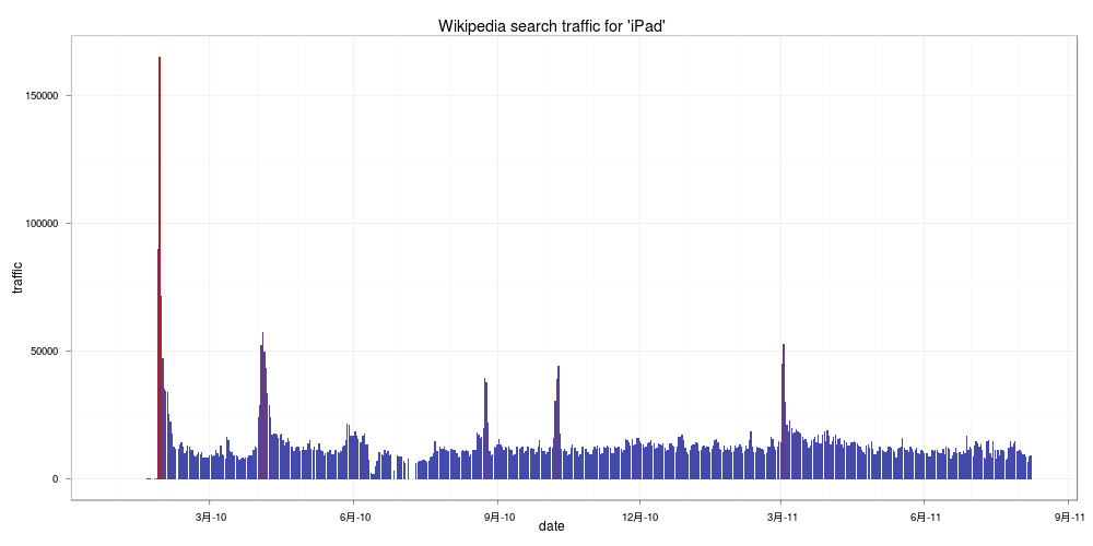
在 2010 年年初 iPad 剛上市時造成轟動,瞬間的查詢量非常高,隨後就降下來,跟 Google 推出的 Android 相比截然不同,也許是兩家公司的行銷手法不一樣所導致的。
R 程式碼
以下是用來分析的 R 函數原始程式碼:
wikiStat <- function (query, lang = 'en',
                      monback = 12,
                      since = Sys.Date() ) {

  #load packages
  require(mondate)
  require(XML)

  namespace <- c("a" = "https://www.w3.org/1999/xhtml")
  wikidata <- data.frame()

  #iterate "monback" number of months back
  for (i in 1:monback) {
    #get number of days in a given month and create a vector
    curdate <- strptime(mondate(since) - (i - 1), "%Y-%m-%d")
    previous <- strptime(mondate(since) - (i - 2), "%Y-%m-%d")
    noofdays <- round(as.numeric(previous - curdate), 0)
    days <- seq(from = 1, to = noofdays, by = 1)

    #build url
    if(curdate$mon + 1 < 10)
    {
      dateurl <- paste(as.character(curdate$year + 1900), "0",
                       as.character(curdate$mon + 1), sep = "")
    }
    else
    {
      dateurl <- paste(as.character(curdate$year + 1900),
                       as.character(curdate$mon + 1), sep = "")
    }

  url <- paste("https://stats.grok.se/",
             lang, '/',
             dateurl, '/',
             query,
             sep = "")
  #get and parse a wikipedia statistics webpage
  wikitree <- xmlTreeParse(url, useInternalNodes=T)

  #find nodes specifying traffic
  traffic <- xpathSApply(wikitree,"//a:li[@class='sent bar']/a:p",
                         xmlValue, namespaces = namespace)

  #edit obtained strings (sometimes its in the format
  # of e.g. 7.5k meaning 7500)
  traffic <- gsub(".", "", traffic)
  traffic <- gsub("k", "00", traffic)
  traffic <- as.numeric(traffic)

  #it seems that there is some kind of a bug in wikipedia statistics
  #and the results are shifted by one day in a month - this is a fix
  if(length(traffic) > noofdays) {
    traffic <- traffic[2:length(traffic)]
  }
  #create daily dates relating to traffic vector
  #and create a dataframe
  days <- seq(from = 1, to = length(traffic), by = 1)
  yearmon <- rep(paste(curdate$year + 1900,
                       curdate$mon + 1, sep = "-"),
                 length(traffic))
  date  <- as.Date(paste(yearmon, days, sep = "-"), "%Y-%m-%d")
  wikidata <- rbind(wikidata, data.frame(date, traffic))
  }

  #remove rows that are missing (due to the bug?)
  wikidata <- wikidata[!is.na(wikidata$date),]

  #return dataframe
  return(wikidata)
}

wikiPlotStat <- function(wikitraffic,
                         title = "Wikipedia statistics") {
  require(ggplot2)

  #create a plot
  wikiplot <- ggplot() + geom_bar(aes(x = date, y = traffic,
                                      fill = traffic),
                                  stat = "identity",
                                  data = wikitraffic) +
                                  opts(title = title)

  #...with no legend and a theme that fits colours of my blog ;)
  wikiplot <- wikiplot + theme_bw() + opts(legend.position = "none")

  return(wikiplot)
}
在使用前要先確定 mondate 與 XML 這兩的套件有沒有裝,若是沒有裝就要先裝才能使用:
install.packages("mondate")
install.packages("XML")
然後就將上面兩個函數的定義複製貼到 R 中執行,或是存成一個 R 程式檔 script.R,使用 source 的方式:
source("script.R")
接下來就可以開始分析了,例如要分析 R_(programming_language) 在 Wikipedia 上面被查詢的狀況:
ar <- wikiStat("R_(programming_language)",
  monback = 45, lang= 'en')
wikiPlotStat(ar,
  "Wikipedia search traffic for 'R (programming language)'")
因為在分析時 R 要從網路上抓取資料,所以分析的時間會比較久,網路比較慢的人要比較有耐心。