TensorFlow 機器學習軟體工具入門教學與範例實作

本篇為 TensorFlow 機器學習軟體工具的入門教學，並實作一個簡單的線性迴歸模型範例。

TensorFlow 是一套由 Google 所發展的開放原始碼機器學習函式庫，其以流程圖的概念呈現整個資料分析流程，在流程圖中的每一個節點都代表一個運算，連接不同節點的連線則代表資料的傳遞，程式設計者可以運用各種不同的運算節點（不同的演算法），組合成適用於各種問題的分析系統，運用 CPU 或 GPU 進行運算。

安裝 TensorFlow

TensorFlow 的安裝方式有很多種，這裡我使用 Docker 的安裝方式，其餘的安裝方法請參考 TensorFlow 官方的文件。

CPU 版 TensorFlow

如果您的電腦沒有 NVIDIA 的 GPU 卡，則可安裝 CPU 版的 TensorFlow。首先安裝好基本的 Docker 環境，再從 Docker Hub 下載 TensorFlow 的 Docker 影像（image）來執行：

docker run -it -p 8888:8888 tensorflow/tensorflow

接著打開 http://localhost:8888/ 這個網址，就可以看到 TensorFlow 的網頁介面了。

GPU 版 TensorFlow

要使用 Docker 運行 GPU 版的 TensorFlow 之前，請先安裝好基本的 Docker 環境，再安裝 NVIDIA Docker 的環境。

接著再從 Docker Hub 下載 TensorFlow 的 Docker 影像（image）來執行：

nvidia-docker run -it -p 8888:8888 tensorflow/tensorflow:latest-gpu

接著打開 http://localhost:8888/ 這個網址，就可以看到 TensorFlow 的網頁介面了。

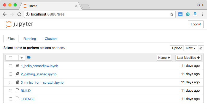
TensorFlow 的網頁介面是採用 Jupyter Notebook 的方式呈現的，這是它的畫面。

Jupyter Notebook

如果想要比較單純的命令列操作介面，可以執行：

nvidia-docker run -it tensorflow/tensorflow:latest-gpu bash

這樣就可以直接開啟一個 bash shell，接著在這個 shell 中執行：

python

即可進入一個有 TensorFlow 的 Python 環境，這種環境適合習慣指令操作的人。

TensorFlow 入門操作

TensorFlow 提供了許多的 API，最底層的 API 就是 TensorFlow Core，其餘較高階的 API 都是以 TensorFlow Core 為基礎所建立的，低階的 TensorFlow Core API 使用上難度比較高，但是可以對模型進行細部的微調，適合機器學習的研究者使用，而較高階的 API 使用上比較簡單，適合一般的使用者來使用。

以下我們將介紹 TensorFlow Core 的用法，在了解 TensorFlow 底層的運作方式之後，再介紹高階 API 的使用方式。

Tensors

TensorFlow 中最基礎的資料類型就是 tensor，它是一種多維度的陣列，其陣列的維度稱為 rank，以下是一些 tensor 的範例：

# 一個 rank 為 0 的 tensor，形狀為 [] 的常數
3

# 一個 rank 為 1 的 tensor，形狀為 [3] 的向量
[1. ,2., 3.]

# 一個 rank 為 2 的 tensor，形狀為 [2, 3] 的矩陣
[[1., 2., 3.], [4., 5., 6.]]

# 一個 rank 為 3 的 tensor，形狀為 [2, 1, 3] 的高維度陣列
[[[1., 2., 3.]], [[7., 8., 9.]]]

在使用 TensorFlow 時，要將 tensorflow 這個 Python 模組匯入：

import tensorflow as tf

接著我們就可以透過這個 tf 使用 TensorFlow 了。

TensorFlow Core 的程式可分為兩大部分：

建立 computational graph。
執行 computational graph。

computational graph 是由許多 TensorFlow 運算節點（nodes）所組成的運算藍圖，每個節點可以接受任意個數的 tensors 作為輸入資料（或是沒有任何輸入也可以），並輸出一個 tensor。

常數節點

constant 節點是一個最簡單的常數節點，它沒有輸入資料，只會輸出其內部儲存的常數，以下是兩個浮點數常數節點範例：

node1 = tf.constant(3.0, dtype = tf.float32)
node2 = tf.constant(4.0) # 預設型別亦為 tf.float32

這裡建立了兩個常數節點，我們可以使用 dtype 來指定資料的型別，若不指定的話預設則為 tf.float32，建立好之後，將其輸出：

print(node1, node2)

(<tf.Tensor 'Const:0' shape=() dtype=float32>, <tf.Tensor 'Const_1:0' shape=() dtype=float32>)

我們將節點輸出之後，並不會直接得到節點的輸出數值，而是看到兩個節點的內部結構，如果要讓節點實際進行運算，必須先建立一個 session，然後在 session 中執行 computational graph：

sess = tf.Session()
print(sess.run([node1, node2]))

這樣就會得到我們所預期的計算結果：

[3.0, 4.0]

我們可以運用加法的節點，把 node1 與 node2 的數值加起來：

node3 = tf.add(node1, node2)
print("node3: ", node3)

('node3: ', <tf.Tensor 'Add:0' shape=() dtype=float32>)

print("sess.run(node3): ",sess.run(node3))

('sess.run(node3): ', 7.0)

我們可以利用 TensorFlow 所附帶的 TensorBoard 功能，以圖型的方式查看 computational graph 的結構。

Placeholder

placeholder 是一種可以讓 computational graph 保留輸入欄位的節點，其允許實際的輸入值留到後來再指定。

a = tf.placeholder(tf.float32)
b = tf.placeholder(tf.float32)
adder_node = a + b  # 加號（+）等同於 tf.add(a, b) 的效果

這種方式其實有點類似定義一個函數，其接受 a 與 b 兩個輸入參數，並且進行加法運算。

接著在執行 computational graph 時，只要在 run 的 feed_dict 參數指定輸入的數值，即可進行運算：

print(sess.run(adder_node, {a: 3, b:4.5}))

7.5

print(sess.run(adder_node, {a: [1,3], b: [2, 4]}))

[ 3.  7.]

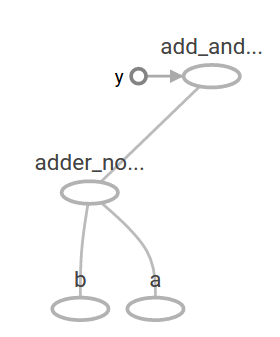
接著我們再把 adder_node 的計算結果拿來再乘以 3.0：

add_and_triple = adder_node * 3.
print(sess.run(add_and_triple, {a: 3, b:4.5}))

22.5

此時的 computational graph 圖形是這樣：

Computational Graph 圖形

Variable

在機器學習的應用上，我們可以讓模型透過 placeholder 輸入各種的資料，而參數的部份我們可以透過 variable 的節點來指定（這樣可以讓參數可以進行訓練）：

W = tf.Variable([.3], dtype=tf.float32)
b = tf.Variable([-.3], dtype=tf.float32)
x = tf.placeholder(tf.float32)
linear_model = W * x + b

常數節點會在呼叫 tf.constant 時就進行初始化，而且其數值是固定的，而 variable 在呼叫 tf.Variable 時並不會進行初始化，若要初始化 variable 要另外執行以下的指令：

init = tf.global_variables_initializer()
sess.run(init)

初始化 variables 之後，就可以將資料放進去這個模型中計算：

print(sess.run(linear_model, {x:[1,2,3,4]}))

[ 0.          0.30000001  0.60000002  0.90000004]

建立好模型之後，我們還會需要評估模型的表現好壞，所以還要定義一個 placeholder y，用於儲存正確的答案：

y = tf.placeholder(tf.float32)

接著使用 tf.square 計算每個誤差的平方，再使用 reduce_sum 把平方後的誤差加總：

squared_deltas = tf.square(linear_model - y)
loss = tf.reduce_sum(squared_deltas)

最後把資料放進去，實際執行：

print(sess.run(loss, {x:[1,2,3,4], y:[,-1,-2,-3]}))

23.66

在學習的過程，我們可以透過調整不同的參數組合，讓誤差值更小。若要調整 variable 的值可以使用 tf.assign：

fixW = tf.assign(W, [-1.])
fixb = tf.assign(b, [1.])
sess.run([fixW, fixb])
print(sess.run(loss, {x:[1,2,3,4], y:[,-1,-2,-3]}))

0.0

當 W 為 -1 且 b 為 1 時，可以獲得最佳解，而接下來的問題就是如何讓程式自動找出最佳解，請繼續閱讀下一頁。

`tf.train` API

在建立好模型之後，接著就是要使用既有的資料對模型進行訓練，TensorFlow 所提供的 optimizers 可以對模型的 variable 進行微調，讓 loss function 達到最小，而最簡單的 optimizer 就是 gradient descent，他會依照 loss function 對個變數的 gradient 方向調整變數，TensorFlow 的 tf.gradients 可以幫助我們計算函數的微分，而 optimizers 也會自動幫我們處理這部分的問題。

首先建立一個 gradient descent optimizer，並指定 loss function：

optimizer = tf.train.GradientDescentOptimizer(0.01)
train = optimizer.minimize(loss)

將原本的變數設定為預設的錯誤組合，然後使用使用迴圈訓練模型，找出最佳的變數組合：

sess.run(init) # 將變數重設為錯誤的組合
for i in range(1000):
  sess.run(train, {x:[1,2,3,4], y:[,-1,-2,-3]})

輸出結果：

print(sess.run([W, b]))

[array([-0.9999969], dtype=float32), array([ 0.99999082], dtype=float32)]

完整的線性迴歸模型程式

前面我們完成了一個簡單的線性迴歸模型程式，其完整的程式碼如下：

import tensorflow as tf

# 模型參數
W = tf.Variable([.3], dtype=tf.float32)
b = tf.Variable([-.3], dtype=tf.float32)

# 輸入與輸出的資料
x = tf.placeholder(tf.float32)
linear_model = W * x + b
y = tf.placeholder(tf.float32)

# loss function
loss = tf.reduce_sum(tf.square(linear_model - y)) # sum of the squares

# optimizer
optimizer = tf.train.GradientDescentOptimizer(0.01)
train = optimizer.minimize(loss)

# training data
x_train = [1, 2, 3, 4]
y_train = [, -1, -2, -3]

# 初始化、重設模型參數
init = tf.global_variables_initializer()
sess = tf.Session()
sess.run(init)

# 最佳化迴圈
for i in range(1000):
  sess.run(train, {x:x_train, y:y_train})

# 輸出結果
curr_W, curr_b, curr_loss = sess.run([W, b, loss], {x:x_train, y:y_train})
print("W: %s b: %s loss: %s"%(curr_W, curr_b, curr_loss))

W: [-0.9999969] b: [ 0.99999082] loss: 5.69997e-11

整個模型以 TensorBoard 畫出來會像這樣：

TensorFlow 線性迴歸模型

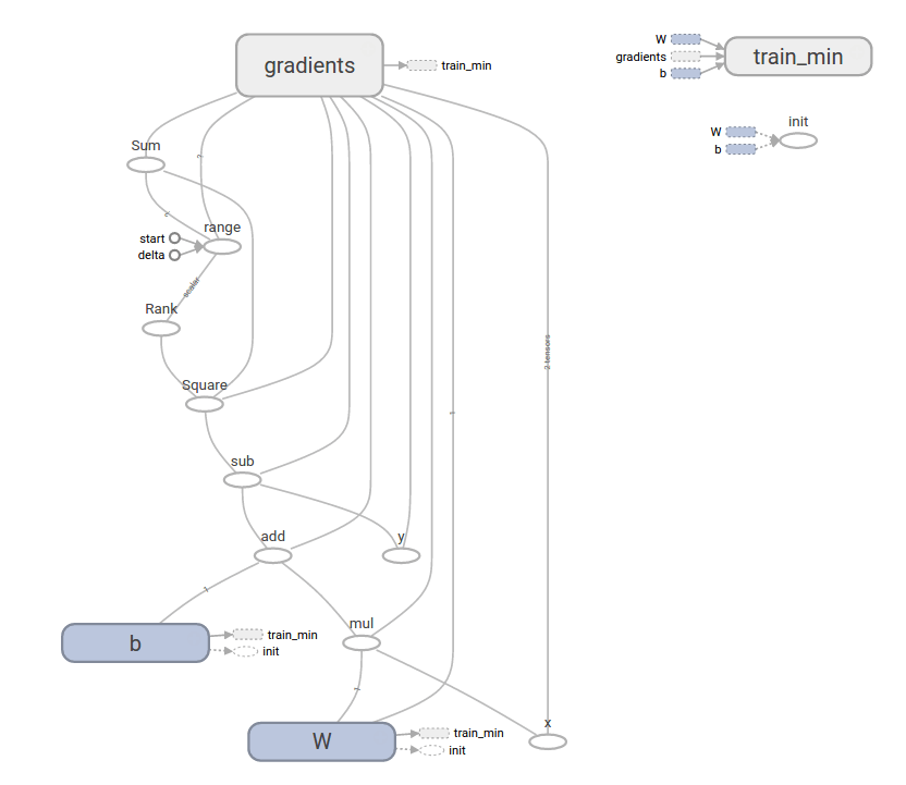
這樣就完成一個基本的機器學習程式了，接下來我們要介紹一些比較高階的 TensorFlow API，使用這些高階 API 可以讓使用者在處理典型的問題上更快速、更簡單。

`tf.contrib.learn`

tf.contrib.learn 是一個高階的 TensorFlow API，可以處理模型的訓練與評估等各種常用的機器學習工作。

以下是使用 tf.contrib.learn 來實作線性迴歸模型的程式碼：

import tensorflow as tf

# NumPy 時常用於載入與整理資料
import numpy as np

# 宣告特徵（fetures），此例中只有一個實數的特徵
features = [tf.contrib.layers.real_valued_column("x", dimension=1)]

# 定義模型，此例使用線性迴歸模型
estimator = tf.contrib.learn.LinearRegressor(feature_columns=features)

# 定義資料，並指定 batch 與 epochs 的大小
x_train = np.array([1., 2., 3., 4.])
y_train = np.array([0., -1., -2., -3.])
x_eval = np.array([2., 5., 8., 1.])
y_eval = np.array([-1.01, -4.1, -7, 0.])
input_fn = tf.contrib.learn.io.numpy_input_fn({"x":x_train}, y_train,
                                              batch_size = 4,
                                              num_epochs = 1000)
eval_input_fn = tf.contrib.learn.io.numpy_input_fn(
    {"x":x_eval}, y_eval, batch_size = 4, num_epochs = 1000)

# 進行模型的訓練
estimator.fit(input_fn = input_fn, steps = 1000)

# 驗證模型
train_loss = estimator.evaluate(input_fn=input_fn)
eval_loss = estimator.evaluate(input_fn=eval_input_fn)
print("train loss: %r"% train_loss)
print("eval loss: %r"% eval_loss)

train loss: {'loss': 2.0923761e-07, 'global_step': 1000}
eval loss: {'loss': 0.0025518893, 'global_step': 1000}

自訂模型

tf.contrib.learn 也允許使用者自訂模型，以下是自訂模型的範例：

import numpy as np
import tensorflow as tf

# 自訂模型
def model(features, labels, mode):
  # 建立線性迴歸模型
  W = tf.get_variable("W", [1], dtype=tf.float64)
  b = tf.get_variable("b", [1], dtype=tf.float64)
  y = W * features['x'] + b
  # loss function 的 sub-graph
  loss = tf.reduce_sum(tf.square(y - labels))
  # 訓練的 sub-graph
  global_step = tf.train.get_global_step()
  optimizer = tf.train.GradientDescentOptimizer(0.01)
  train = tf.group(optimizer.minimize(loss),
                   tf.assign_add(global_step, 1))
  # 使用 ModelFnOps 將我們建立的 subgraphs 包裝好
  return tf.contrib.learn.ModelFnOps(
      mode=mode, predictions=y,
      loss=loss,
      train_op=train)

# 定義模型
estimator = tf.contrib.learn.Estimator(model_fn=model)

# 定義資料，並指定 batch 與 epochs 的大小
x_train = np.array([1., 2., 3., 4.])
y_train = np.array([0., -1., -2., -3.])
x_eval = np.array([2., 5., 8., 1.])
y_eval = np.array([-1.01, -4.1, -7, 0.])
input_fn = tf.contrib.learn.io.numpy_input_fn({"x": x_train}, y_train, 4, num_epochs=1000)

# 進行模型的訓練
estimator.fit(input_fn=input_fn, steps=1000)

# 驗證模型
train_loss = estimator.evaluate(input_fn=input_fn)
eval_loss = estimator.evaluate(input_fn=eval_input_fn)
print("train loss: %r"% train_loss)
print("eval loss: %r"% eval_loss)

train loss: {'loss': 2.0923761e-07, 'global_step': 1000}
eval loss: {'loss': 0.0025518893, 'global_step': 1000}

安裝 TensorFlow#

CPU 版 TensorFlow#

GPU 版 TensorFlow#

TensorFlow 入門操作#

Tensors#

常數節點#

Placeholder#

Variable#

tf.train API#

完整的線性迴歸模型程式#

tf.contrib.learn#

自訂模型#