SymPy 是一個可以進行數學代數運算的 Python 模組,他的發展目標是一個完整的電腦代數系統,而此模組完全都是使用 Python 寫成的,所以不需要依賴其他的函式庫。
準備 SymPy 環境
在 Ubuntu 或 Debian Linux 中若要安裝 SymPy,可以直接使用 apt 安裝:
sudo apt-get install python-sympy
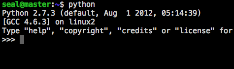
裝完之後,接著就可以執行 Python 了:
python
進入 Python 的互動式模式(interactive mode)之後,就會看到三個大於符號(>>>),這就是 Python 的主要命令提示字元(primary prompt)。
如果是只要使用 SymPy 的功能,可以使用 isympy 這個指令,這是專門為了 SymPy 而設計的互動式介面,其實跟 Python 的互動式環境一樣,但是 isympy 會在一開始設定一些基本的變數與環境,讓使用起來更方便。
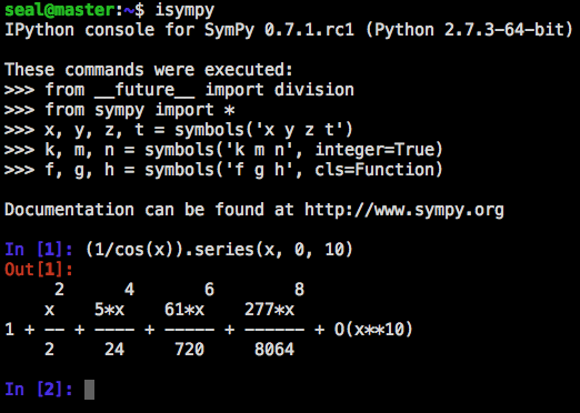
藍色的 In 就是輸入指令的地方,輸出則是紅色的 Out,後面中括弧中的數字是自動編上去的行號。
如果不想那麼麻煩安裝 SymPy,也可以直接使用 SymPy Live,直接在網頁上運行 SymPy,其實更方便,開啓網頁後,左下方就可以直接輸入 Python 指令了。
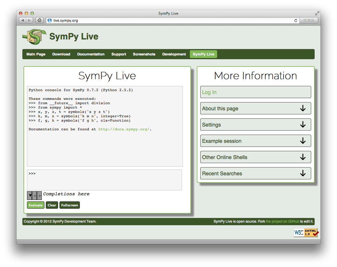
而 SymPy Live 的環境就跟上面的 isympy 差不多,一開始就會把一些基本的變數與環境設定好。這種線上版本的排版比一般終端機還要漂亮,我們在這裡執行相同的指令,與上面的 isympy 比較一下。
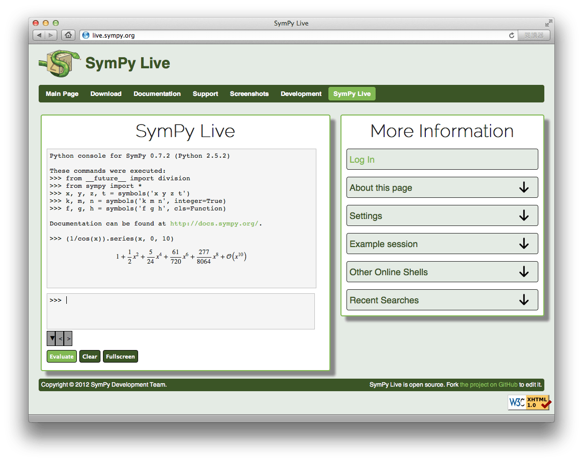
因為 SymPy Live 是用 MathJax 來顯示數學式子的,所以看起來很漂亮,幾乎跟 LaTeX 的排版差不多。若是沒什麼特別需求,用這個就很棒了,省去安裝的麻煩。
開始使用 SymPy
接著就可以輸入 Python 指令了,在使用之前要先載入 sympy 這個 Python 模組,輸入:
>>> from sympy import *
輸入完這行指令之後,記得按下 Enter 鍵,正常的話應該沒有什麼訊息出現。這個指令是將 sympy 中所有的東西都載入進來,如果一開始執行了這行指令,之後所有的 import 步驟都可以省略,而如果不想一次載入所有的東西也可以,那就按照下面的 import 作法,需要使用時才載入。
接著就可以來使用 SymPy 了,首先來介紹一些基本的使用方式。在 SymPy 中的數值分為三種類型,分別為浮點數(Float)、有理數(Rational)與整數(Integer)。有理數是由兩個整數相除所得到的數值,例如 Rational(1, 2) 則代表 1/2:
>>> from sympy import Rational
>>> a = Rational(1, 2)

>>> a
1/2

>>> a*2
1

>>> Rational(2)**50/Rational(10)**50
1/88817841970012523233890533447265625
在使用浮點數與整數運算時(尤其是除法)要注意所使用的數值是 SymPy 數值或是原生的 Python 數值,若是使用一般原生的 Python 數值,相除的結果會是浮點數,若在 isympy 中則會使用 __future__ 中的 division 進行除法運算。
>>> 1/2
0.5
若是在舊版的 Python 2 中,division 沒有被 import,則結果會被 truncated:
>>> 1/2
0
這兩種狀況都是使用 Python 原生的數值,不是 SymPy 數值,在大部分的狀況下,在使用 SymPy 時都會使用 SymPy 數值,所以其實可以使用這樣的方式簡化程式碼:
>>> R = Rational
>>> R(1, 2)
1/2

>>> R(1)/2
1/2
最後一個指令中 R(1) 會得到一個 Rational 數值,再除以原生的 Python 數值 2,得到的結果也是一個 Rational 數值。
在數學上有一些常數,例如圓周率(pi)與尤拉常數(e),在 SymPy 中也有支援,在運算時他會以符號的方式進行運算,也就是說 1 + pi 不會計算成浮點數 4.14,而會保持 1 + pi 這個形式,若是要算出實際的浮點數,可以使用 evalf() 這個函數。
>>> from sympy import pi, E
>>> pi**2
pi**2

>>> pi.evalf()
3.14159265358979

>>> (pi + E).evalf()
5.85987448204884
數學上的無限大(infinity)在 SymPy 中也有,表示方式為兩個 o(看起來就像是無限大的寫法)。
>>> from sympy import oo
>>> oo
oo

>>> oo + 1
oo
符號(Symbol)與代數運算
SymPy 與其他的 CAS(Computer Algebra System)不同,在 SymPy 中所有的變數都要經過宣告才能使用:
>>> from sympy import Symbol
>>> x = Symbol('x')
>>> y = Symbol('y')
第二行是將 Python 變數 x 指定為 SymPy Symbol。
在 sympy.abc 中有預先定義一些 Symbol(包涵一些以希臘字母命名的 Symbol)。
>>> from sympy.abc import x, theta
若要建立多個 Symbol 可以使用 symbols 與 var 兩個函數,兩個函數作用相同,都可以接受 range notation,但 var 會自動將建立的 Symbol 加入命名空間(namespace)。
>>> from sympy import symbols, var
>>> a, b, c = symbols('a,b,c')
>>> d, e, f = symbols('d:f')
>>> var('g:h')
(g, h)
>>> var('g:2')
(g0, g1)
建立了 Symbol 之後,就可以使用它們進行代數運算了。
>>> x + y + x - y
2*x

>>> (x + y)**2
(x + y)**2

>>> ((x + y)**2).expand()
x**2 + 2*x*y + y**2
Symbol 亦可被替換為其他的 Symbol 或是數值。
>>> ((x + y)**2).subs(x, 1)
(y + 1)**2

>>> ((x + y)**2).subs(x, y)
4*y**2

>>> ((x + y)**2).subs(x, 1 - y)
1
apart(expr, x) 函數可以處理 partial fraction decomposition。
>>> from sympy import apart
>>> from sympy.abc import x, y, z
>>> 1/( (x + 2)*(x + 1) )
       1
---------------
(x + 1)*(x + 2)

>>> apart(1/( (x + 2)*(x + 1) ), x)
    1       1
- ----- + -----
  x + 2   x + 1

>>> (x + 1)/(x - 1)
x + 1
-----
x - 1

>>> apart((x + 1)/(x - 1), x)
      2
1 + -----
    x - 1
而 together(expr, x) 則與 apart 相反,將所有的項結合在一起。
>>> from sympy import together
>>> together(1/x + 1/y + 1/z)
x*y + x*z + y*z
---------------
     x*y*z

>>> together(apart((x + 1)/(x - 1), x), x)
x + 1
-----
x - 1

>>> together(apart(1/( (x + 2)*(x + 1) ), x), x)
       1
---------------
(x + 1)*(x + 2)
微積分(Calculus)
SymPy 也可以用於微積分的計算,這裡介紹在微積分中常用的運算。
SymPy 提供了ㄧ個 limit(function, variable, point) 函數可以計算函數的極限值。下面的這個指令可以計算 sin(x) 函數在 x 趨近於零的極限值。
>>> from sympy import limit, Symbol, sin, oo
>>> x = Symbol('x')
>>> limit(sin(x)/x, x, 0)
1
亦可計算無限大的極限值:
>>> limit(x, x, oo)
oo

>>> limit(1/x, x, oo)
0

>>> limit(x**x, x, 0)
1
再舉一個更複雜的例子:
>>> limit((1+1/x)**x, x, oo)
E

>>> limit((x**3-1)/(x**2-1), x, 1)
3/2

>>> limit(E**x/(1-x**3), x, 0)
1
這裡的 E 就是數學上的尤拉常數。
diff(func, var) 這個函數可以計算微分(differentiation):
>>> from sympy import diff, Symbol, sin, tan
>>> x = Symbol('x')
>>> diff(sin(x), x)
cos(x)

>>> diff(sin(2*x), x)
2*cos(2*x)

>>> diff(tan(x), x)
   2
tan (x) + 1
我們可以用下面的指令確認這個答案是正確的:
>>> from sympy import limit
>>> from sympy.abc import delta
>>> limit((tan(x + delta) - tan(x))/delta, delta, 0)
   2
tan (x) + 1
更高階的微分可以使用 diff(func, var, n):
>>> diff(sin(2*x), x, 1)
2*cos(2*x)

>>> diff(sin(2*x), x, 2)
-4*sin(2*x)

>>> diff(sin(2*x), x, 3)
-8*cos(2*x)
SymPy 的 Symbol 可以用 .series(var, point, order) 轉成泰勒展開式(Taylor series):
>>> from sympy import Symbol, cos
>>> x = Symbol('x')
>>> cos(x).series(x, 0, 10)
     2    4     6      8
    x    x     x      x      / 10
1 - -- + -- - --- + ----- + Ox  /
    2    24   720   40320
>>> (1/cos(x)).series(x, 0, 10)
     2      4       6        8
    x    5*x    61*x    277*x     / 10
1 + -- + ---- + ----- + ------ + Ox  /
    2     24     720     8064
另外一個例子:
>>> from sympy import Integral, pprint
>>> y = Symbol("y")
>>> e = 1/(x + y)
>>> s = e.series(x, 0, 5)
>>> print(s)
1/y - x/y**2 + x**2/y**3 - x**3/y**4 + x**4/y**5 + O(x**5)
>>> pprint(s)
          2    3    4
1   x    x    x    x     / 5
- - -- + -- - -- + -- + Ox /
y    2    3    4    5
    y    y    y    y
summation(f, (i, a, b)) 這個函數可以計算 f 函數從 a 到 b 的加總,也就是:
summation 函數如果沒辦法計算出總和,就會顯示原本的加總公式。下面是一些範例:
>>> from sympy import summation, oo, symbols, log
>>> i, n, m = symbols('i n m', integer=True)
>>> summation(2*i - 1, (i, 1, n))
 2
n
>>> summation(1/2**i, (i, 0, oo))
2
>>> summation(1/log(n)**n, (n, 2, oo))
  oo
 ___
   `
       -n
  /   log (n)
 /__,
n = 2
>>> summation(i, (i, 0, n), (n, 0, m))      3    2
m    m    m
-- + -- + -
6    2    3
>>>  from sympy.abc import x
>>>  from sympy import factorial
>>>  summation(x**n/factorial(n), (n, 0, oo))
 x
e
在積分方面,SymPy 支援定積分(definite integration)與不定積分(indefinite integration),而積分的計算是使用 integrate() 函數。
>>> from sympy import integrate, erf, exp, sin, log, oo, pi, sinh, symbols
>>> x, y = symbols('x,y')
>>> integrate(6*x**5, x)
 6
x
>>> integrate(sin(x), x)
-cos(x)
>>> integrate(log(x), x)
x*log(x) - x
>>> integrate(2*x + sinh(x), x)
 2
x  + cosh(x)
更複雜的例子:
>>> integrate(exp(-x**2)*erf(x), x)
  ____    2
/ pi *erf (x)
--------------
      4
計算定積分:
>>> integrate(x**3, (x, -1, 1))
0
>>> integrate(sin(x), (x, 0, pi/2))
1
>>> integrate(cos(x), (x, -pi/2, pi/2))
2
瑕積分(improper integral)也同樣支援:
>>> integrate(exp(-x), (x, 0, oo))
1
>>> integrate(log(x), (x, 0, 1))
-1
複數(Complex numbers)
SymPy 也可以處理複數,Symbol 亦可以指定屬性(attribute),例如:real、positive 或 complex 等,指定屬性會影響其運算的結果。
>>> from sympy import Symbol, exp, I
>>> x = Symbol("x") # a plain x with no attributes
>>> exp(I*x).expand()
 I*x
e
>>> exp(I*x).expand(complex=True)
   -im(x)               -im(x)
I*e      *sin(re(x)) + e      *cos(re(x))
>>> x = Symbol("x", real=True)
>>> exp(I*x).expand(complex=True)
I*sin(x) + cos(x)
三角函數(Trigonometric)
>>> from sympy import asin, asinh, cos, sin, sinh, symbols, I
>>> x, y = symbols('x,y')
>>> sin(x + y).expand(trig=True)
sin(x)*cos(y) + sin(y)*cos(x)
>>> cos(x + y).expand(trig=True)
-sin(x)*sin(y) + cos(x)*cos(y)
>>> sin(I*x)
I*sinh(x)
>>> sinh(I*x)
I*sin(x)
>>> asinh(I)
I*pi
----
 2
>>> asinh(I*x)
I*asin(x)
>>> sin(x).series(x, 0, 10)
     3     5     7       9
    x     x     x       x       / 10
x - -- + --- - ---- + ------ + Ox  /
    6    120   5040   362880

>>> sinh(x).series(x, 0, 10)
     3     5     7       9
    x     x     x       x       / 10
x + -- + --- + ---- + ------ + Ox  /
    6    120   5040   362880

>>> asin(x).series(x, 0, 10)
     3      5      7       9
    x    3*x    5*x    35*x     / 10
x + -- + ---- + ---- + ----- + Ox  /
    6     40    112     1152

>>> asinh(x).series(x, 0, 10)
     3      5      7       9
    x    3*x    5*x    35*x     / 10
x - -- + ---- - ---- + ----- + Ox  /
    6     40    112     1152
Spherical Harmonics
>>> from sympy import Ylm
>>> from sympy.abc import theta, phi
>>> Ylm(1, 0, theta, phi)
  ___
/ 3 *cos(theta)
----------------
        ____
    2*/ pi

>>> Ylm(1, 1, theta, phi)
   ___  I*phi
-/ 6 *e     *sin(theta)
------------------------
            ____
        4*/ pi

>>> Ylm(2, 1, theta, phi)
   ____  I*phi
-/ 30 *e     *sin(theta)*cos(theta)
------------------------------------
                  ____
              4*/ pi
階乘(factorials)與 Gamma 函數
>>> from sympy import factorial, gamma, Symbol
>>> x = Symbol("x")
>>> n = Symbol("n", integer=True)

>>> factorial(x)
x!

>>> factorial(n)
n!

>>> gamma(x + 1).series(x, 0, 3) # i.e. factorial(x)
                      /          2     2
                    2 |EulerGamma    pi |    / 3
1 - EulerGamma*x + x *|----------- + ---| + Ox /
                           2         12/
Zeta 函數
>>> from sympy import zeta
>>> zeta(4, x)
zeta(4, x)

>>> zeta(4, 1)
  4
pi
---
 90

>>> zeta(4, 2)
       4
     pi
-1 + ---
      90

>>> zeta(4, 3)
         4
  17   pi
- -- + ---
  16    90
多項式(polynomials)
>>> from sympy import assoc_legendre, chebyshevt, legendre, hermite
>>> chebyshevt(2, x)
   2
2*x  - 1

>>> chebyshevt(4, x)
   4      2
8*x  - 8*x  + 1

>>> legendre(2, x)
   2
3*x    1
---- - -
 2     2

>>> legendre(8, x)
      8         6         4        2
6435*x    3003*x    3465*x    315*x     35
------- - ------- + ------- - ------ + ---
  128        32        64       32     128

>>> assoc_legendre(2, 1, x)
        __________
       /    2
-3*x*/  - x  + 1

>>> assoc_legendre(2, 2, x)
     2
- 3*x  + 3

>>> hermite(3, x)
   3
8*x  - 12*x
微分方程(Differential Equations)
>>> from sympy import Function, Symbol, dsolve
>>> f = Function('f')
>>> x = Symbol('x')
>>> f(x).diff(x, x) + f(x)
        2
       d
f(x) + ---(f(x))
         2
       dx

>>> dsolve(f(x).diff(x, x) + f(x), f(x))
f(x) = C1*sin(x) + C2*cos(x)
代數方程式(Algebraic Equations)
>>> from sympy import solve, symbols
>>> x, y = symbols('x,y')
>>> solve(x**4 - 1, x)
[-1, 1, -I, I]

>>> solve([x + 5*y - 2, -3*x + 6*y - 15], [x, y])
{x: -3, y: 1}
線性代數(Linear Algebra)
建立矩陣可以使用 Matrix 類別:
>>> from sympy import Matrix, Symbol
>>> Matrix([[1, 0], [0, 1]])
[1  0]
[    ]
[0  1]
矩陣中亦可包含 Symbol:
>>> x = Symbol('x')
>>> y = Symbol('y')
>>> A = Matrix([[1, x], [y, 1]])
>>> A
[1  x]
[    ]
[y  1]

>>> A**2
[x*y + 1    2*x  ]
[                ]
[  2*y    x*y + 1]
Pattern Matching
使用 .match() 方法並配合 Wild 類別可以對 Symbol 進行比對,例如抓取某一項的係數等,這個方法會傳回一個 dictionary,例如:
>>> from sympy import Symbol, Wild
>>> x = Symbol('x')
>>> p = Wild('p')
>>> (5*x**2).match(p*x**2)
{p: 5}

>>> q = Wild('q')
>>> (x**2).match(p*x**q)
{p: 1, q: 2}
如果沒有找到指定的 pattern,則會傳回 None:
>>> print (x + 1).match(p**x)
None
亦可使用 Wild 的 exclude 參數排除指定的比對結果:
>>> p = Wild('p', exclude=[1, x])
>>> print (x + 1).match(x + p) # 1 is excluded
None
>>> print (x + 1).match(p + 1) # x is excluded
None
>>> print (x + 1).match(x + 2 + p) # -1 is not excluded
{p_: -1}
輸出顯示(Printing)
SymPy 的運算結果可以用好幾種不同的方式輸出,一般預設的方式是使用 str(expression) 的方式,例如:
>>> from sympy import Integral
>>> from sympy.abc import x
>>> print x**2
x**2
>>> print 1/x
1/x
>>> print Integral(x**2, x)
Integral(x**2, x)
而 pprint() 函數(pretty printing)可以將結果以 ascii-art 的方式「畫」出來,例如:
>>> from sympy import Integral, pprint
>>> from sympy.abc import x
>>> pprint(x**2)
 2
x
>>> pprint(1/x)
1
-
x
>>> pprint(Integral(x**2, x))
  /
 |
 |  2
 | x  dx
 |
/
若您的系統有安裝 unicode 字型,則 pprint() 函數預設就會使用它,亦可使用 use_unicode 參數自行設定。
>>> pprint(Integral(x**2, x), use_unicode=True)
⌠
⎮  2
⎮ x  dx
⌡
下面示範將 pprint() 設定為預設的輸出函數:
$ python
Python 2.5.2 (r252:60911, Jun 25 2008, 17:58:32)
[GCC 4.3.1] on linux2
Type "help", "copyright", "credits" or "license" for more information.
>>> from sympy import init_printing, var, Integral
>>> init_printing(use_unicode=False, wrap_line=False, no_global=True)
>>> var("x")
x
>>> x**3/3
 3
x
--
3
>>> Integral(x**2, x) #doctest: +NORMALIZE_WHITESPACE
  /
 |
 |  2
 | x  dx
 |
/
使用 Python 輸出:
>>> from sympy.printing.python import python
>>> from sympy import Integral
>>> from sympy.abc import x
>>> print python(x**2)
x = Symbol('x')
e = x**2
>>> print python(1/x)
x = Symbol('x')
e = 1/x
>>> print python(Integral(x**2, x))
x = Symbol('x')
e = Integral(x**2, x)
使用 LaTeX 輸出:
>>> from sympy import Integral, latex
>>> from sympy.abc import x
>>> latex(x**2)
x^{2}
>>> latex(x**2, mode='inline')
$x^{2}$
>>> latex(x**2, mode='equation')
begin{equation}x^{2}end{equation}
>>> latex(x**2, mode='equation*')
begin{equation*}x^{2}end{equation*}
>>> latex(1/x)
frac{1}{x}
>>> latex(Integral(x**2, x))
int x^{2}, dx
使用 MathML 輸出:
>>> from sympy.printing.mathml import mathml
>>> from sympy import Integral, latex
>>> from sympy.abc import x
>>> print mathml(x**2)
<apply><power><ci>x</ci><cn>2</cn></power></apply>
>>> print mathml(1/x)
<apply><power><ci>x</ci><cn>-1</cn></power></apply>
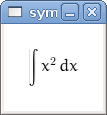
使用 Pyglet:
>>> from sympy import Integral, preview
>>> from sympy.abc import x
>>> preview(Integral(x**2, x))
如果系統上有安裝 pyglet 的話,就會跳出這個視窗: